Morphology
pyKNEEr computes two quantitative metrics to characterize femoral cartilage morphology:
Thickness, calculated in two steps:
Separation of subcondral surface and articular surface of the cartilage
Calculation of the distance between the two surfaces using a nearest neighbor method
Volume, calculated as the volume of the cartilage mask multiplied by the voxel volume
Note
You can calculate cartilage thickness and volume independently although their computations are implemented in the same notebook
Input: Image folder list
For the demo images, the input file is image_list_morphology.txt, which contains:
[1] ./segmented
[2] 01_DESS_01_prep_fc.mha
where:
Line 1: Input folder, containing the cartilage masks
Line 2: Name of cartilage mask
Tip
When using your own data:
Customize
image_list_morphology.txtwith path and names of your own binary masks
Executing morphology.ipynb
To compute femoral cartilage morphology:
Launch Jupyter notebook
In File Browser, navigate to
morphology.ipynb, open it, and:Customize the input variables :
n_of_cores(How do I choose the number of cores?)output_file_name_thicknessoutput_file_name_volume
Follow the instructions in the notebook ```{note} Cartilage thickness and volume are calculated independently, so it is not necessary to calculate thickness before calculating the volume`
Save your notebook at the end of the process
Output: Surfaces, thicknesses, and volumes
The outputs are in the folder .morphology. For each subject, the outputs are:
*_boneCart.txt: Subchondral surface of the cartilage as a points cloud. Each row corresponds to a point, and the three columns correspond to the x, y, and z coordinates*_artiCart.txt: Articular surface of the cartilage as a points cloudthickness_ID.txt: List of thicknesses in mm associated to the surface pointsIDis the algorithm chosen to calculate cartilage thickness:Nearest neighbor calculated on the femur surface
Nearest neighbor calculated on the articular surface
volume.txt: Cartilage volume in \(mm^3\)
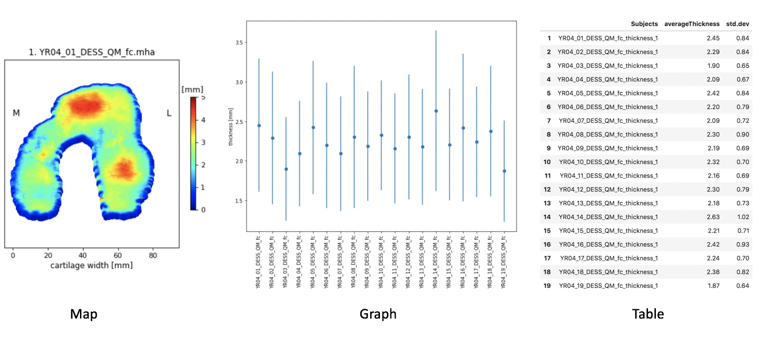
Visualization: Map, graph, and table
Cartilage thickness is visualized as:
Map: Thickness values are a colormap on the cartilage surface, flattened after interpolation to a cylinder [1]. The same flattening algorithm is used to visualize subcondral and articular cartilage after splitting
Graph: Dots represent the average value of cartilage thickness per image and bars represent the standard deviation
Table: Thickness average and standard deviation, also saved as
.csvfile for subsequent analysis
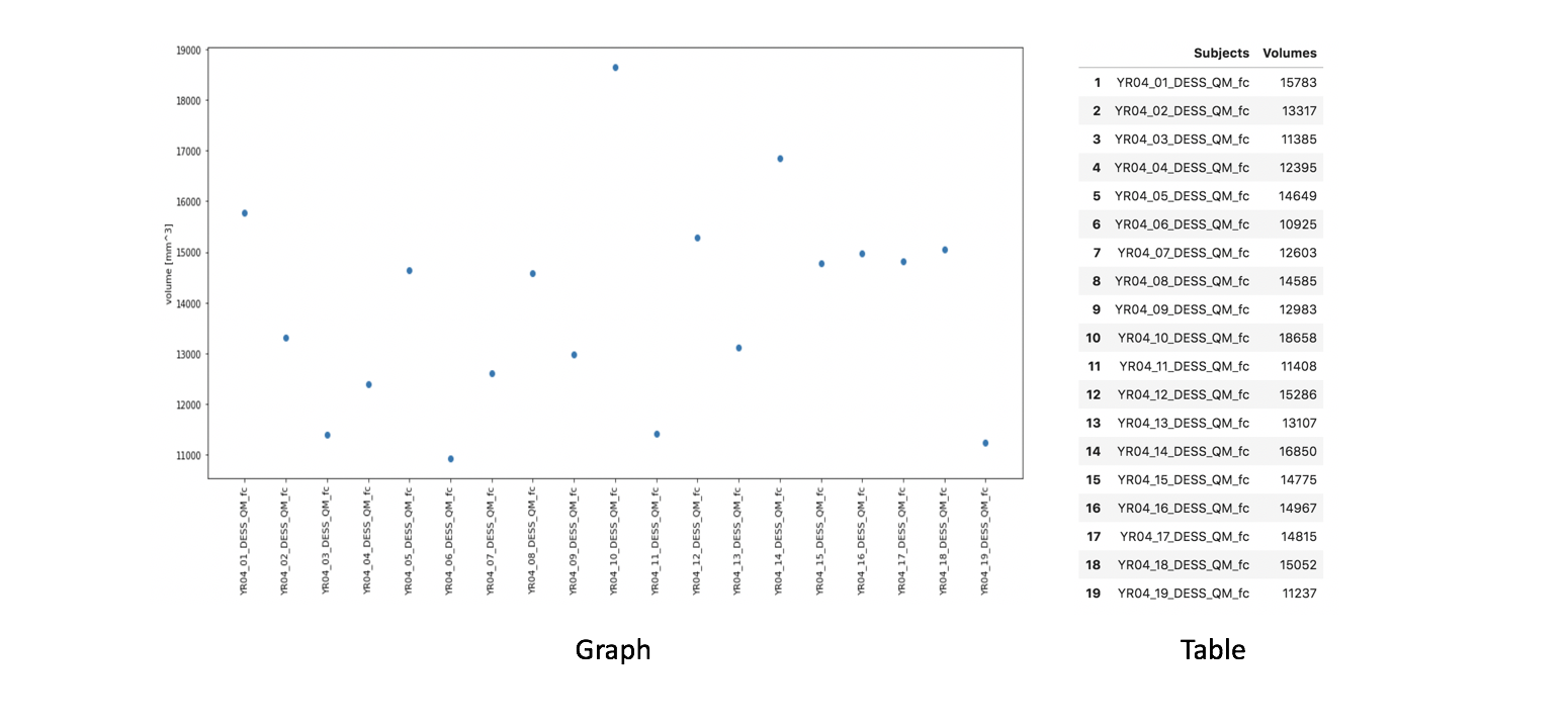
Cartilage volume is visualized as:
Graph: Dots represent volume per image
Table: Volume values, also saved as
.csvfile for subsequent analysis
References
[1] Monu U.D., Jordan C.D., Samuelson B.L., Hargreaves B.A., Gold G.E., McWalter E.J. Cluster analysis of quantitative MRI T2 and T1ρ relaxation times of cartilage identifies differences between healthy and ACL-injured individuals at 3T. Osteoarthritis Cartilage. Apr;25(4):513-520. 2017.