Segmentation¶

pyKNEEr computes atlas-based segmentation, which is based on registration, using elastix [1]. In registration there are a reference (or target) image and a moving (or floating) image, which is warped to the reference image. The reference image is already segmented, whereas the moving image has to be segmented.

In pyKNEEr, atlas-based segmentation has three steps:

The moving image is registered to the reference image though transformations
The transformations are inverted
The inverted transformations are applied to the reference mask to obtain the moving mask

These steps are applied:

To the femur to align the moving image to the reference image, and guide femoral cartilage segmentation
To the femoral cartilage to obtain the segmented image

Important

The current method does not take into account segmentation accuracy at the bone-cartilage interface. The femur alignment is used to guide cartilage segmentation, and femur segmentation is a byproduct of the workflow.

In pyKNEEr, there are three segmentation modalities:

New subject: Segmentation of single images, baseline images in longitudinal studies, or high-resolution images in multimodal acquisitions
Multimodal: Segmentation of images acquired with different protocols, where the highest resolution image has already been segmented as new subject
Longitudinal: Segmentation of followup images, where the baseline image has already been segmented as new subject

For the execution, the differences among the three modalities are:

The reference image
The structure of the input file
The variable modality in segmentation_sa.ipynb

New subject segmentation¶

Reference image¶

The reference image is the same for all the images to be segmented

In the folder reference, the reference image is in the folder newsubject, which contains:

reference.mha: Reference image for the atlas-based segmentation
reference_f.mha: Femur mask of the reference image
reference_fc.mha: Femoral cartilage mask of the reference image.

This reference was found with a convergence study on 19 segmented images

Tip

When using your own data:

You can use the same reference image contained in the demo dataset: copy the files reference.mha, reference_f.mha, and reference_fc.mha to your reference/newsubject folder
You can use a different reference image: copy your new reference image, femur mask, and femoral cartilage mask to the reference/newsubject folder, making sure you rename the files as reference.mha, reference_f.mha, and reference_fc.mha
If you want to find a reference image from an already segmented dataset, you can run pyKNEEr convergence study

Input: Image list¶

For the demo images, the input file is image_list_newsubject.txt, which contains:

  [1] ./reference/newsubject
  [2] ./preprocessed/
  [3] r reference.mha
  [4] m 01_DESS_01_prep.mha

where:

Line 1: Reference folder, containing the reference image and its masks
Line 2: Preprocessed file folder, containing the preprocessed files
Line 3: Reference image, indicated as r
Line 4: Moving images, indicated as m

Tip

When using your own data:

Customize image_list_newsubject.txt with the paths and the names of your images
There is no limit to the number of moving m images

Executing `segmentation_sa_ns.ipynb`¶

To segment the data:

Launch Jupyter notebook
In File Browser, navigate to segmentation_sa_ns.ipynb, open it, and:
- Customize the input variable n_of_cores (How do I choose the number of cores?)
- Notice that variable modality is set to newsubject
- Follow the instructions in the notebook
Save your notebook at the end of the process

Output: Segmented images¶

The masks are in the folder segmented. For each subjects, the outputs are:

*_prep_fc.mha (e.g. 01_DESS_01_prep_fc.mha): Binary mask of the femoral cartilage
*_prep_f.mha (e.g. 01_DESS_01_prep_f.mha): Binary mask of the femur, a byproduct of the registration

Note

Intermediate registration steps are saved in the folder registered
If you are not interested in analysis from deformations, you can delete the folder after your computations
If you want to compute further analysis, the folders registered/subject_name contain:
- fc_spline.mha (intersubject and longitudinal segmentation) or f_rigig.mha (multimodal segmentation), which contain the moving image warped to the reference. They can be used for analysis such as voxel-based relaxometry
- TransformParameters.xxx.txt, which contain transformation values. They can be used for PCA or other analysis. For their use, we forward to the elastix manual

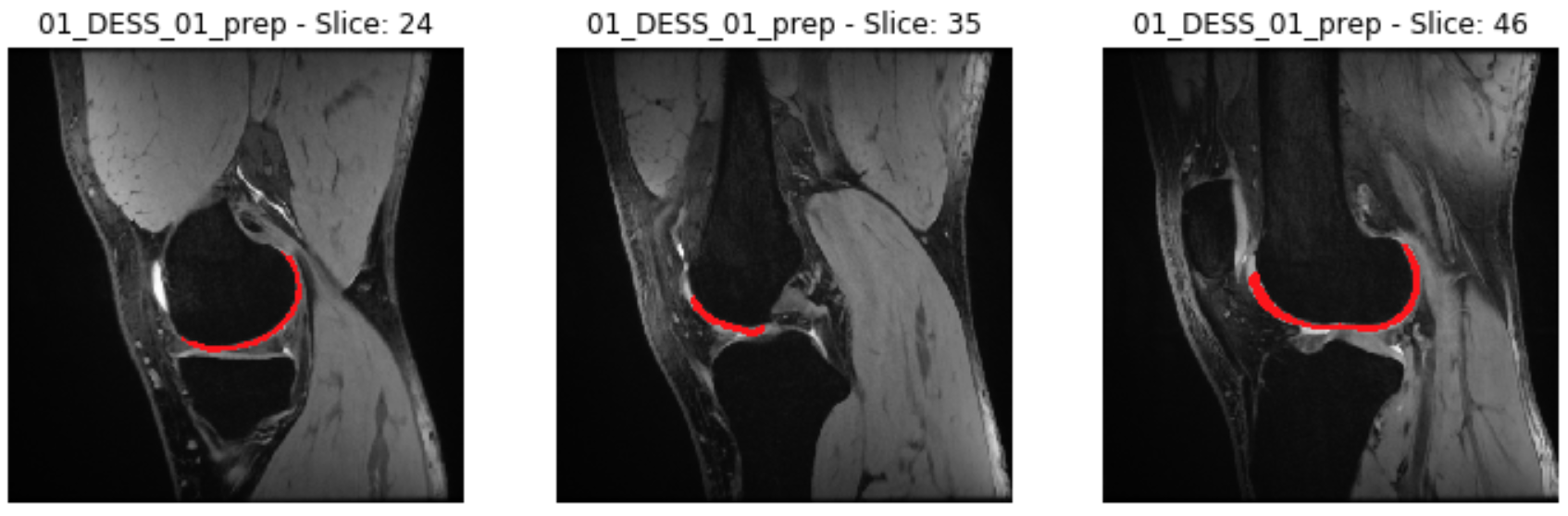
Visualization: Superimposing cartilage mask onto the MR image¶

For a qualitative check, for each subject we visualize three 2D slices of the intensity image (*_prep.mha) overlapped by the corresponding slices of the cartilage mask (*_prep_fc.mha), similarly to this figure:

For a 3D check, consider using a medical image software such as ITK-SNAP, which allows visualizing the overlap of an image and its mask

Multimodal segmentation¶

Reference image¶

For each acquisition at lower resolution (e.g. CubeQuant), the reference image is a high-resolution image of the same subject (e.g. DESS), which must have been previously segmented as a newsubject.

In the folder reference, create the folder multimodal, and copy:

The high-resolution image: 01_DESS_01_prep.mha from the folder preprocessed
The high-resolution femur mask: 01_DESS_01_prep_f.mha from the folder segmented
The high-resolution femoral cartilage mask: 01_DESS_01_prep_fc.mha from the folder segmented

This step will be simplified in future versions of pyKNEEr

Tip

When using your own data:

In the folder reference create the folder multimodal
Copy the high-resolution images to be used as a references, together with their femur mask and femoral cartilage mask

Input: Image list¶

For the demo images, the input file is image_list_multimodal.txt, which contains:

  [1] ./reference/multimodal
  [2] ./preprocessed/
  [3] r 01_DESS_01_prep.mha
  [4] m 01_cubeQuant_01_prep.mha

where:

Line 1: Reference folder, containing the baseline images used as reference
Line 2: Preprocessed file folder, containing the preprocessed images
Line 3: Reference (high res) image, indicated as r
Line 4: Moving (low res) image, indicated as m

Tip

When using your own data:

Customize image_list_multimodal.txt with the paths and the names of your images

In case of several images to segment, write high-resolution images r and low-resolution images m in a coupled manner:

  [1] ./reference/longitudinal
  [2] ./preprocessed/
  [3] r subject1_HRes_prep.mha
  [4] m subject1_LRes_prep.mha
  [5] r subject2_HRes_prep.mha
  [6] m subject2_LRes_prep.mha
  [7] r subject3_HRes_prep.mha
  [8] m subject3_LRes_prep.mha
  [9] etc.

Execution, Output, and Visualization¶

Execution:

To segment the data, apply the instructions above to the notebook segmentation_sa_mm.ipynb. Note that the variable modality is set to multimodal

Output and visualization:

Follow the instructions above to know the output and how to visualize the results

Longitudinal¶

For this segmentation modality, we do not provide a demo example but only instructions as it is very similar to multimodal segmentation

Reference image¶

For each followup image, the reference image is the corresponding baseline image, which must have been previously segmented as a new subject

In the folder reference, create the folder longitudinal, and for each image copy:

The baseline image: BL_prep.mha
The baseline femur mask: BL_prep_f.mha
The baseline femoral cartilage mask: BL_prep_fc.mha

This step will be simplified in future versions of pyKNEEr.

Input: Image list¶

Create the file image_list_longitudinal.txt, which will contain:

  [1] ./reference/longitudinal
  [2] ./preprocessed/
  [3] r subject1_BL_prep.mha
  [4] m subject1_FU_prep.mha
  [5] r subject2_BL_prep.mha
  [6] m subject2_FU_prep.mha
  [7] r subject3_BL_prep.mha
  [8] m subject3_FU_prep.mha

where:

Line 1: Reference folder, containing the the baseline images used as reference
Line 2: Preprocessed file folder, containing the preprocessed files of the corresponding followup images
Odd lines from 3 to 7: Reference (baseline) images, indicated as r
Even lines 4 to 8: Moving (followup) images, indicated as m

Execution, Output, and Visualization¶

Execution:

To segment the data, apply the instructions above. Set the variable modality to longitudinal

Output and visualization:

Follow the instructions above to know the output and how to visualize the results

Segmentation Plus¶

pyKNEEr includes notebooks to find the reference image and evaluate segmentation quality

These two steps are not included in the demo for sake of simplicity

Finding reference image¶

In this convergence study, the new reference is the image of the dataset whose vector field is the closest to the average of the vector fields of the dataset. The study runs until convergence or for a fixed amount of iterations

Note

To run this convergence study all the images of the dataset must already have a femur mask }

The Jupyter notebook to find a reference image is find_reference.ipynb

Picking random seeds¶

To determine the image that you are going to use as reference, we recommend a random generator function with a fixed seed to make the reference selection reproducible. The code is here.

You can run several convergence study in parallel to confirm you find the same reference image independently from the starting seed

Input: Image list¶

Data required are MR images of the knee that have segmented femurs because:

the registration is guided by the femur mask
the average vector field is calculated in the femur mask
the comparison between the average vector field and each image vector field is performed in the femur mask

In you data folder, create a folder called findReference and add the preprocessed images of the dataset with their masks:

- subject1_prep.mha
- subject1_f.mha
- subject2_prep.mha
- subject2_f.mha
- subject3_prep.mha
- subject3_f.mha

File nomenclature has be as follows:

The file name root of image and corresponding mask has to be the same
The image name has to end in _prep.mha
The mask name must end in _f.mha

Create the input file:

[1] ./findReference
[2] r subject2_prep.mha
[3] m subject1_prep.mha
[4] m subject2_prep.mha
[5] m subject3_prep.mha
[6] m etc.

where:

Line 1: findReference folder, containing all the images of the dataset
Line 2: Reference image, indicated as r
Line 3-5: Moving images, indicated as m

Note that in this example subject2_prep.mha is both the reference and an image of the dataset, because we want to include it as a possible candidate for being the final reference

If you run multiple studies, created the input file for every seed image, adapting the reference (r) file name

Executing findReference.ipynb¶

For each seed image, in findReference.ipynb customize input_file_name and n_of_cores

Launch findReference.ipynb. It will run until convergence or until the number of iterations reaches 10 (If you run the source code, you can change the number of iterations in the file find_reference_for_nb.py, function find_reference, variable maxIterationNo)

Output: Convergence plot¶

The output of the computation is a convergence plot. The graph can reach a plateau or can be zig-zagged. In this last case, choose the reference with the lowest error (y-axis). If the graph shows less than 10 iterations it means that the current reference image is the same as the one in the previous loop.

Segmentation quality¶

You can quantify segmentation quality when a ground truth segmentation is present, whereas you can evaluate segmentation quality only visually when a ground truth segmentation is not available

The metrics we use to evaluate segmentation quality are:

Measures of overlap agreement: Dice coefficient, Jaccard coefficient, and volume similarity, which quantify the overlap between ground truth segmentations and pyKNEEr segmentations
Measure of surface distance: Average of the Euclidean distances between ground truth segmentations and pyKNEEr segmentations

The Jupyter notebook to evaluate segmentation is segmentation_quality.ipynb

Input: Image list¶

Create the input file:

[1] ./segmented
[2] ./segmented_groundTruth
[3] s subject1_prep_fc.mha
[4] g subject1_groundTruth_fc.mha
[5] s subject2_prep_fc.mha
[6] g subject2_groundTruth_fc.mha
[7] m etc.

where:

Line 1: Segmented folder, containing the masks obtained with pyKNEEr
Line 2: Ground truth folder, containing ground truth masks
Lines 3,5: Segmentations obtained with pyKNEEr, indicated as s
Lines 4,6: Ground truth segmentations, indicated as g

Execution, Output, and Visualization¶

Execution:

In segmentation_quality.ipynb, customize input_file_name, output_file_name_overlap, and output_file_name_distances, and execute

Output and visualization:

Results will be visualized as graphs and tables, and will be saved in the .csv files for possible subsequent analysis

References¶

[1] Klein S., Staring M., Murphy K., Viergever M.A., Pluim J.P.W. elastix: A Toolbox for Intensity-Based Medical Image Registration. IEEE Transactions on Medical Imaging. vol. 29, no. 1, pp. 196 - 205, January. 2010.

Segmentation¶

New subject segmentation¶

Reference image¶

Input: Image list¶

Executing segmentation_sa_ns.ipynb¶

Output: Segmented images¶

Visualization: Superimposing cartilage mask onto the MR image¶

Multimodal segmentation¶

Reference image¶

Input: Image list¶

Execution, Output, and Visualization¶

Longitudinal¶

Reference image¶

Input: Image list¶

Execution, Output, and Visualization¶

Segmentation Plus¶

Finding reference image¶

Picking random seeds¶

Input: Image list¶

Executing findReference.ipynb¶

Output: Convergence plot¶

Segmentation quality¶

Input: Image list¶

Execution, Output, and Visualization¶

References¶

Executing `segmentation_sa_ns.ipynb`¶